5. Processes
The processes are the core of a model. LIAM2 supports two kinds of processes: assignments, which change the value of a variable (predictor) using an expression, and actions which don’t (but have other effects).
For each entity (for example, “household” and “person”), the block of processes starts with the header “processes:”. Each process then starts at a new line with an indentation of four spaces.
5.1. Assignments
Assignments have the following general format:
processes:
    variable1_name: expression1
    variable2_name: expression2
    ...
The variable_name will usually be one of the variables defined in the fields block of the entity but, as we will see later, it is not always necessary.
In this case, the name of the process equals the name of the endogenous variable. Process names have to be unique for each entity. See the section about procedures if you need to have several processes which modify the same variable.
To run the processes, they have to be specified in the “processes” section of the simulation block of the file. This explains why the process names have to be unique for each entity.
example
entities:
    person:
        fields:
            - age: int
        processes:
            age: age + 1
simulation:
    processes:
        - person: [age]
    ...
5.2. Temporary variables
All fields declared in the “fields” section of the entity are stored in the output file. Often you need a variable only to store an intermediate result during the computation of another variable.
In LIAM2, you can create a temporary variable at any point in the simulation by simply having an assignment to an undeclared variable. Their value will be discarded at the end of the period.
example
person:
    fields:
        # period and id are implicit
        - age:      int
        - agegroup: int

processes:
    age: age + 1
    agediv10: trunc(age / 10)
    agegroup: agediv10 * 10
    agegroup2: agediv10 * 5
In this example, agediv10 and agegroup2 are temporary variables. In this particular case, we could have bypassed the temporary variable, but when a long expression occurs several times, it is often cleaner and more efficient to express it (and compute it) only once by using a temporary variable.
5.3. Actions
Since actions don’t return any value, they do not need a variable to store that result, and they only ever need the condensed form:
processes:
    process_name: action_expression
    ...
example
processes:
    remove_deads: remove(dead)
5.4. Procedures
A process can consist of sub-processes, in that case we call it a procedure. Processes within a procedure are executed in the order they are declared.
Sub-processes each start on a new line, again with an indentation of four spaces and a -.
So the general setup is:
processes:
    variable_name: expression
    process_name2: action_expression
    process_name3:
        - subprocess_31: expression
        - subprocess_32: expression
In this example, there are three processes, of which the first two do not have sub-processes. The third process is a procedure which consists of two sub-processes. If it is executed, subprocess_31 will be executed and then subprocess_32.
Contrary to normal processes, sub-processes (processes inside procedures) names do not need to be unique. In the above example, it is possible for subprocess_31 and subprocess_32 to have the same name, and hence simulate the same variable. Procedure names (process_name3) does not directly refer to a specific endogenous variable.
example
processes:
    ageing:
        - age: age * 2 # in our world, people age strangely
        - age: age + 1
        - agegroup: trunc(age / 10) * 10
The processes on age and agegroup are grouped in ageing. In the simulation block you specify the ageing-process if you want to update age and agegroup.
By using procedures, you can actually make building blocks or modules in the model.
5.4.1. Local (temporary) variables
Temporary variables defined/computed within a procedure are local to that procedure: they are only valid within that procedure. If you want to pass variables between procedures you have to make them global by defining them in the fields section.
(bad) example
person:
    fields:
        - age: int

    processes:
        ageing:
            - age: age + 1
            - isold: age >= 150   # isold is a local variable

        rejuvenation:
            - age: age – 1
            - backfromoldage: isold and age < 150  # WRONG !
In this example, isold and backfromoldage are local variables. They can only be used in the procedure where they are defined. Because we are trying to use the local variable isold in another procedure in this example, LIAM 2 will refuse to run, complaining that isold is not defined.
5.4.2. Actions
Actions inside procedures don’t even need a process name.
example
processes:
    death_procedure:
        - dead: age > 150
        - remove(dead)
5.5. Expressions
Expressions can either compute new values for existing individuals, or change the number of individuals by using the so-called life-cycle functions.
5.5.1. simple expressions
Let us start with a simple increment; the following process increases the value of a variable by one each simulation period.
age: age + 1
The name of the process is age and what it does is increasing the variable age of each individual by one, each period.
- Arithmetic operators: +, -, *, /, ** (exponent), % (modulo)
Note
An integer divided by an integer returns a float. For example “1 / 2” will evaluate to 0.5 instead of 0 as in many programming languages. If you are only interested in the integer part of that result (for example, if you know the result has no decimal part), you can use the trunc function:
agegroup5: 5 * trunc(age / 5)
- Comparison operators: <, <=, ==, !=, >=, >
- Boolean operators: and, or, not
Note
Starting with version 0.6, you do not need to use parentheses when you mix boolean operators with other operators.
inwork: workstate > 0 and workstate < 5
to_give_birth: not gender and age >= 15 and age <= 50
is now equivalent to:
inwork: (workstate > 0) and (workstate < 5)
to_give_birth: not gender and (age >= 15) and (age <= 50)
- Conditional expressions: if(condition, expression_if_true, expression_if_false)
example
agegroup_civilstate: if(age < 50,
                        5 * trunc(age / 5),
                        10 * trunc(age / 10))
Note
The if function always requires three arguments. If you want to leave a variable unchanged if a condition is not met, use the variable in the expression_if_false:
# retire people (set workstate = 9) when aged 65 or more
workstate: if(age >= 65, 9, workstate)
You can nest if-statements. The example below retires men (gender = True) over 64 and women over 61.
workstate: if(gender,
              if(age >= 65, 9, workstate),
              if(age >= 62, 9, workstate))
# could also be written like this:
workstate: if(age >= if(gender, 65, 62), 9, workstate)
5.5.2. globals
Globals can be used in expressions in any entity. LIAM2 currently supports two kinds of globals: tables and multi-dimensional arrays. They both need to be imported (see the Importing data section) and declared (see the globals section) before they can be used.
Globals tables come in two variety: those with a PERIOD column and those without.
The fields in a globals table with a PERIOD column can be used like normal (entity) fields except they need to be prefixed by the name of their table:
myvariable: mytable.MYINTFIELD * 10
the value for INTFIELD is in fact the value INTFIELD has for the period currently being evaluated.
There is a special case for the periodic table: its fields do not need to be prefixed by “periodic.” (but they can be, if desired).
- retirement_age: if(gender, 65, WEMRA)
- workstate: if(age >= retirement_age, 9, workstate)
This changes the workstate of the individual to retired (9) if the age is higher than the required retirement age in that year.
Another way to use globals from a table with a PERIOD column is to specify explicitly for which period you want them to be evaluated. This is done by using tablename.FIELDNAME[period_expr], where period_expr can be any expression yielding a valid period value. Here are a few artificial examples:
workstate: if(age >= WEMRA[2010], 9, workstate)
workstate: if(age >= WEMRA[period - 1], 9, workstate)
workstate: if(age >= WEMRA[year_of_birth + 60], 9, workstate)
Globals tables without a PERIOD column can only be used with the second syntax, and in that case LIAM2 will not automatically subtract the “base period” from the index, which means that to access a particular row, you have to use its row index (0 based).
Globals arrays can simply be used like a normal field:
myvariable: MYARRAY * 2
5.5.3. mathematical functions
- log(expr): natural logarithm (ln)
- exp(expr): exponential
- abs(expr): absolute value
- round(expr[, n]): returns the rounded value of expr to specified n (number of digits after the decimal point). If n is not specified, 0 is used.
- trunc(expr): returns the truncated value (by dropping the decimal part) of expr as an integer.
- clip(x, a, b): returns a if x < a, x if a < x < b, b if x > b.
- min(x, a), max(x, a): the minimum or maximum of x and a.
5.5.4. aggregate functions
- count([condition]): count individuals
It counts the individuals in the current entity. If a (boolean) condition is given, it only counts the ones satisfying that condition. For example, count(male and age >= 18) will produce the number of men in the sample who are eighteen years old or older.
Note
count() can be used without any argument: count() will return the total number of individuals in the sample for the current entity.
- sum(expr[, filter=condition][, skip_na=True]): sum of an expression
It computes the sum of any expression over all individuals of the current entity. If a filter (boolean condition) is given, it only takes into account the individuals satisfying the filter. For example sum(earnings) will produce the sum of the earnings of all persons in the sample, while sum(earnings, age >= 30) will produce the sum of the earnings of all persons in the sample who are 30 or older. skip_na determines whether missing values (nan) are discarded before the computation or not. It defaults to True.
Note
sum and count are exactly equivalent if their only argument is a boolean variable (eg. count(age >= 18) == sum(age >= 18)).
- avg(expr[, filter=condition][, skip_na=True]): average
- std(expr[, filter=condition][, skip_na=True]): standard deviation
- min(expr[, filter=condition][, skip_na=True]): min
- max(expr[, filter=condition][, skip_na=True]): max
- median(expr[, filter=condition][, skip_na=True]): median
- percentile(expr, percent[, filter=condition][, skip_na=True]): percentile
- gini(expr[, filter=condition][, skip_na=True]): gini
- all(condition1[, filter=condition2]): is condition True for all?
Returns True if all individuals who satisfy the optional condition2 also satisfy condition1, False otherwise. Note that all(condition1, filter=condition2) is equivalent to all(condition1 and condition2).
- any(condition1[, filter=condition2]): is condition True for any?
Returns True if any individual who satisfy the optional condition2 also satisfy condition1, False otherwise. Note that any(condition1, filter=condition2) is equivalent to any(condition1 and condition2).
5.5.5. link methods
(one2many links)
- link.count([filter]) - counts the number of related individuals
- link.sum(expr[, filter]) - compute the sum of an expression over the related individuals
- link.avg(expr[, filter]) - compute the average of an expression over the related individuals
- link.min(expr[, filter]) - compute the minimum of an expression over the related individuals
- link.max(expr[, filter]) - compute the maximum of an expression over the related individuals
example
entities:
    household:
        fields:
            # period and id are implicit
            - nb_persons: {type: int, initialdata: false}
        links:
            persons: {type: one2many, target: person, field: household_id}

        processes:
            household_composition:
                - nb_persons: persons.count()
                - nb_students: persons.count(workstate == 1)
                - nb_children: persons.count(age <= 17)
                - avg_age: persons.avg(age)
5.5.6. temporal functions
lag(expr[, num_periods][, missing=value): value at previous period.
expr: any expression.
num_periods: optional argument specifying the number of periods to go back to. This can be either a constant or a scalar expression. Defaults to 1.
missing: the value to return for individuals which were not present in the past period. By default, it returns the missing value corresponding to the type of the expression: -1 for an integer expression, nan for a float or False for a boolean.
example
lag(age)            # the age each person had last year, -1 if newborn
lag(age, missing=0) # the age each person had last year, 0 if newborn
avg(lag(age))       # average age that the current population had last year
lag(avg(age))       # average age of the population of last year
lag(age, 2)         # the age each person had two years ago (-1 for
                    # newborns)
lag(lag(age))       # this is equivalent (but slightly less efficient)
value_for_period(expr, period[, missing=value]): value at a specific period
expr: any expression.
period: the period used to evaluate the expression. This can be either a constant or a scalar expression.
missing: the value to return for individuals which were not present in the period. By default, it returns the missing value corresponding to the type of the expression: -1 for an integer expression, nan for a float or False for a boolean.
example
value_for_period(inwork and not male, 2002)duration(expr): number of consecutive period the expression was True
examples
duration(inwork and (earnings > 2000))
duration(educationlevel == 4)
tavg(expr): average of an expression since the individual was created
example
tavg(income)tsum(expr): sum of an expression since the individual was created
5.5.7. random functions
- uniform: random numbers with a uniform distribution [0,1)
- normal: random numbers with a normal distribution
- randint: random integers between bounds
example
# a random variable with the stdev derived from errsal
normal(loc=0.0, scale=std(errsal))
randint(0, 10)
5.5.7.1. choice
Monte Carlo or probabilistic simulation is a method for iteratively evaluating a deterministic model using sets of random numbers as inputs. In microsimulation, the technique is used to simulate changes of state dependent variables. Take the simplest example: suppose that we have an exogenous probability of an event happening, P(x=1), or not P(x=0). Then draw a random number u from an uniform [0,1) distribution. If, for individual i, ui < P(x=1), then xi=1. If not, then xi=0. The expected occurrences of x after, say, 100 runs is then P(x=1) * 100 and the expected value is 1xP(1)+0xP(0)=P(1). This type of simulation hinges on the confrontation between a random variable and an exogenous probability.
In LIAM 2, such a probabilistic simulation is called a choice process. Suppose i=1..n choice options, each with a probability prob_option_i. A choice expression then has the following form:
choice([option_1, option_2, ..., option_n],
       [prob_option_1, prob_option_2, ..., prob_option_n])
Note that both the list of options and their probabilities are between []’s. The options can be of any numeric type.
A simple example of a process using a choice expression is the simulation of the gender of newborns (51% males and 49% females), as such:
gender: choice([True, False], [0.51, 0.49])
In the current version of LIAM 2, it is not possible to combine a choice with alignment.
Here is a more complex example of a process using choice. Suppose we want to simulate the work status (blue collar worker or white collar worker) for all working individuals. We want to assign 1 or 2 to their collar variable based on their sex and level of education (education_level=2, 3, 4). We could write our process as follow:
collar_process:
    - no_collar: WORKING and collar == -1
    - collar: if(no_collar and (education_level == 2),
                 if(gender,
                    choice([1, 2], [0.836, 0.164]),
                    choice([1, 2], [0.687, 0.313]) ),
                 collar)
    - collar: if(no_collar and (education_level == 3),
                 if(gender,
                    choice([1, 2], [0.643, 1 - 0.643]),
                    choice([1, 2], [0.313, 1 - 0.313]) ),
                 collar)
    - collar: if(no_collar and (education_level == 4),
                 if(gender,
                    choice([1, 2], [0.082, 1 - 0.082]),
                    choice([1, 2], [0.039, 1 - 0.039]) ),
                 collar)
The procedure collar_process has collar as the key endogenous variable and has four sub-processes.
The first sub-process defines a local variable no_collar, which will be used to select those that the procedure should apply to. These are all the workers that do not have a value for collar.
The next three sub-processes simulate the actual collar variable. If one meets the above no_collar filter and has the lowest level of education (2), then one has a probability of about 83.6% (men) and 68.7% (women) of being a blue collar worker. If one has “education_level” equal to 3, the probability of being a blue collar worker is lower (64.3% for men and 31.3% for women), etc.
5.5.8. Regressions
5.5.8.1. logit_score
The logit of a number p between 0 and 1 is given by the formula:
logit(p) = log(p / (1 - p))
Its inverse, the logistic function has the interesting property that it can convert any real number into a probability.
logistic(a) = 1 / (1 + exp(-a))
The logit_score function is a logistic with a random part:
logit_score(a) = logistic(a - logit(u))
where u is a random number from an uniform distribution [0, 1).
logit_score is very useful in behavioural equations. A behavioural equation starts by creating a score that reflects the risk p*i of an event occuring. A typical usage is as follow:
- score_variable: if(condition_1,
                     logit_score(logit_expr_1),
                     if(condition_2,
                        logit_score(logit_expr_2),
                        -1))
However, the nested structure can make things less readable if you have many different conditions. In that case, one would prefer the following longer form:
process_name:
    # initialise the score to -1
    - score_variable: -1

    # first condition
    - score_variable: if(condition_1,
                         logit_score(logit_expr_1),
                         score_variable)
    # second condition
    - score_variable: if(condition_2,
                         logit_score(logit_expr_2),
                         score_variable)

    # ... other conditions ...
In a first sub-process, a variable score_variable is set equal to -1, because this makes it highly unlikely that the event will happen to those not included in the conditions for which the logit is applied.
Next, subject to conditions condition_1 and condition_2, this score (risk) is simulated on the basis of estimated logits. Note that by specifying the endogenous variable score_variable without any transformation in the “else” conditions of the if functions makes sure that the score variable is not manipulated by a sub-process it does not pertain to.
When the score is known, it can be either used as-is:
- event_happened: uniform() < score_variable
or in combination with an alignment (see below).
5.5.8.2. align
Now that we have computed a score (risk) for an event happening, we might want to use alignment so the number of events occuring per category matches a proportion defined externaly.
There are different ways to choose which individuals are taken. The methodology used for now by LIAM 2 is called “alignment by sorting”, that is, for each category, the N individuals with the highest scores are selected.
The score computation is not done internally by the align() function, but is rather computed by an expression given by the modeller. One will usually use logit_score() to compute it, but it can be computed in any other way a modeller choose.
Note
It is usually a good idea to include a random component (like in logit_score) in the score expression because otherwise the individuals with the smaller scores will never be selected.
To know more about the alignment process reading “Evaluating Alignment Methods in Dynamic Microsimulation Models”, by Li and O’Donoghue is advised.
An alignment expression takes the following general form:
align(score,
      proportions
      [, filter=conditions]
      [, take=conditions]
      [, leave=conditions]
      [, expressions=expressions]
      [, possible_values=pvalues]
      [, frac_need="uniform"|"round"|"cutoff"])
For example, it could look like:
- unemp: align(unemp_score,
               'al_p_unemployed_m.csv',
               filter=not ISINWORK and (age > 15) and (age < 65),
               take=ISUNEMPLOYED,
               leave=ISSTUDENT or ISRETIRED)
Now let us examine each argument in turn:
score: it must be an expression (or a simple variable) returning a numerical value. It will be used to rank individuals. One will usually use logit_score() to compute the score, but it can be computed in any other way a modeller choose. Note that the score is not modified in any way within the align() function, so if one wants a random factor, it should be added manually (or through the use of a function like logit_score which includes one).
proportions: the target proportions for each category. This argument can take many forms. The most common one will probably be a string holding the name of a file containing the alignment data (like in the example above) but it can be any of the following:
a single scalar, for aligning with a constant proportion.
a list of scalars, for aligning with constant proportions per category.
an expression returning a single scalar.
an expression returning an n-dimensional array. expressions and possible values will be retrieved from that array, so you can simply use:
align(score_expr, array_expr)a list of expressions returning scalars [expr1, expr2].
a string treated as a filename. That file should be in the “array” format described in the Importing data section. In that case, the proportions, expressions (column names) and possible values are read from that file. The “fname” argument which used to be the way to define this is still supported for backward compatibility.
There is no technical restriction on names for files containing alignment data but, by convention, they usually use the following pattern: start with the prefix al_ followed by the name of the endogenous variable and a suffix _m or _f, depending on gender.
filter: an expression specifying which individuals to take into account for the alignment. Note that if the align() function is used inside an if() expression, its filter is adjusted accordingly (“anded” with the filter of the if() expression). For example:
- aligned: if(condition,
              align(score_expr1, 'filename1.csv'),
              align(score_expr2, 'filename2.csv'))
is equivalent to:
- aligned1: align(score_expr1, 'filename1.csv', filter=condition) - aligned2: align(score_expr2, 'filename2.csv', filter=not condition) - aligned: if(condition, aligned1, aligned2)take: an expression specifying individuals which should always be selected, regardless of their score. This argument should be used with care as those individuals will be selected unconditionally, even if that means overflowing the number of individuals desired to satisfy the alignment.
Suppose that the alignment specifies that 10 individuals should experience a certain event, and that there are 3 individuals who meet the conditions specified in the take. Then these 3 individuals will be selected a priori (irrespective of their score) and the alignment process will select the remaining 7 candidates from the rest of the sample.
A “softer” alternative can be easily achieved by setting a very high score for individuals to be taken first.
leave: an expression specifying individuals which should never be selected, regardless of their score. This argument should be used with care as those individuals will never be selected, even if that cause the target number of individuals for some categories to not be reached.
A “softer” alternative can be easily achieved by setting a very low score for individuals to be taken last.
Note
Note that even if the score for an individual is -1 (or any other negative number), it can still be selected by the alignment expression. This happens when there are not enough candidates (selected by the filter) to meet the alignment needs.
expressions: specify the expressions used to partition the individuals into the different alignment categories. If proportions is a file name, the column names declared in the file are used by default, but they can be overridden using this argument. For example:
align(0.0, 'al_p_dead.csv', expressions=[gender, age + 1])possible_values: specify the different values for each of the expressions in the expressions argument that should be evaluated. The combination of the different lists of possible values will form all the alignment categories. For example:
align(0.0, proportions=[0.1, 0.2, 0.3, 0.4], expressions=[gender, age < 50], possible_values=[[False, True], [False, True]])frac_need: control how “fractional needs” are handled. This argument can take any of three values: “uniform” (default), “cutoff” or “round”.
“uniform” draws a random number (u) from an uniform distribution and adds one individual if u < fractional_need. “uniform” is the default behavior.
“round” simply rounds needs to the nearest integer. In other words, one individual is added for a category if the fractional need for that category is >= 0.5.
“cutoff” tries to match the total need as closely as possible (at the expense of a slight loss of precision for individual categories) by searching for the “cutoff point” that yields:
count(frac_need >= cutoff) == sum(frac_need)
In practice alignment data is often separate for men and women. In that case, one will usually use the following form:
- variable: if(condition,
               if(gender,
                  align(score_expr, 'filename_m.csv'),
                  align(score_expr, 'filename_f.csv')),
               False)
Since LIAM2 supports alignment with any number of dimensions, one could also merge both data files in a single file with one more dimension and use a single align() expression:
- variable: if(condition,
               align(score_expr, 'filename_m_and_f.csv'),
               False)
# or even
- variable: align(score_expr, 'filename_m_and_f.csv', filter=condition)
In the example below describes the process of getting (or keeping) a job:
inwork:
    - work_score: -1
    # men
    - work_score: if(ISMALE and ACTIVEAGE and ISINWORK,
                     logit_score(-0.196599 * age + 0.0086552 * age **2 - 0.000988 * age **3
                                 + 0.1892796 * ISMARRIED + 3.554612),
                     work_score)
    - work_score: if(ISMALE and ACTIVEAGE and (ISUNEMPLOYED or ISOTHERINACTIVE),
                     logit_score(0.9780908 * age - 0.0261765 * age **2 + 0.000199 * age **3
                                 - 12.39108),
                     work_score)
    # women
    - work_score: if(ISFEMALE and ACTIVEAGE and ISINWORK,
                     logit_score(-0.2740483 * age + 0.0109883 * age **2 - 0.0001159 * age **3
                                 - 0.0906834 * ISMARRIED + 3.648706),
                     work_score)
    - work_score: if(ISFEMALE and ACTIVEAGE and (ISUNEMPLOYED or ISOTHERINACTIVE),
                     logit_score(0.8217638 * age - 0.0219761 * age **2 + 0.000166 * age **3
                                 - 0.5590975 * ISMARRIED - 10.48043),
                     work_score)

    - work: if(ACTIVEAGE,
               if(ISMALE,
                  align(work_score, 'al_p_inwork_m.csv',
                        leave=ISSTUDENT or ISRETIRED),
                  align(work_score, 'al_p_inwork_f.csv',
                        leave=ISSTUDENT or ISRETIRED)),
               False)
The first sub process illustrates a “soft leave” by setting the score variable work_score to -1. This makes sure that the a priori selection probability is very low (but not zero, as in the case of leave conditions) for those who satisfy the filter of the alignment but for which a score is not explicitly specified the subsequent processes.
Next come four if conditions, separating the various behavioural equations to the sub-sample they pertain to. The first two conditions pertain to men and respectively describe the probability of keeping a job and getting a job. The next two conditions describe the same transitions but for women.
The last sub-process describes the alignment process itself. Alignment is applied to individuals between the age of 15 and 65. The input-files of the alignment process are ‘al_p_inwork_m.csv’ and ‘al_p_inwork_f.csv’. The alignment process uses as input the scores simulated previously, and the information in the alignment files and sets the boolean variable work. No “take” or “leave” conditions are used in this case.
5.5.8.3. align_abs
align_abs is equivalent to align(), except that it aligns to absolute numbers instead of proportions. It also supports a few additional arguments to work on a linked entity.
The general form of align_abs is :
align_abs(score,
          need,
          [, filter=conditions]
          [, take=conditions]
          [, leave=conditions]
          [, expressions=expressions]
          [, possible_values=pvalues]
          [, frac_need="uniform"|"round"|"cutoff"]
          [, link=link_name]
          [, secondary_axis=column_name]
          [, errors="default"|"carry"])
In addition to all the arguments supported by align(), align_abs() also supports an optional “link” argument, which makes it work on a linked entity.
Here is a description of the arguments specific to align_abs:
link: must be the name of a one2many link. When the link argument is used, the groups (given by the alignment file or in the expressions argument) are evaluated on the linked entity and the needs are expressed in terms of that linked entity. When the link argument is in effect, align_abs uses the “Chenard” algorithm.
This can be used, for example, to take as many households as necessary trying to get as close as possible to a particular distribution of persons.
secondary_axis: name of an axis which will influence rel_need when the subtotal for that axis is exceeded. See total_by_sex in Chenard. secondary_axis can only be used in combination with the link argument and it must be one of the alignment columns.
errors: if set to ‘carry’, the error for a period (difference between the number of individuals aligned and the target for each category) is stored and added to the target for the next period. In the current version of LIAM2, errors can only be used in combination with the link argument.
example
test_align_link:
    # this is a procedure defined at the level of households
    - num_persons: persons.count()
    - total_population: sum(num_persons)

    # MIG_PERCENT is a simple float periodic global
    - num_migrants: total_population * MIG_PERCENT

    # MIG is a 3d array: age - gender - period but we want only the
    # 2d array for this period.
    # currently, we need to manually compute the index (0-based)
    # for the current period in the array. We know the first
    # period in our array is 2000, so the index for the current
    # period is: "period - 2000"
    # period is the last dimension of the array and we do not
    # want to modify other dimensions, so we use ":" for those
    # dimensions.
    - mig_period: MIG[:,:,period - 2000]

    # Distribute total desired migrants, by age and gender
    - need: num_migrants * mig_period

    # households have a 50% chance to be candidate for immigration
    - is_candidate: uniform() < 0.5

    # apply alignment, using the number of persons in each household
    # as a score, so that households with more persons are tried first
    # as this gives better results.
    - aligned: align_abs(num_persons, need,
                         filter=is_candidate,
                         link=persons, secondary_axis=gender,
                         errors='carry')
5.5.8.4. logit_regr
logit_regr is a shortcut form to call logit_score and “evaluate whether the event happened” in a single function. Thus, the function returns a boolean: True for individuals which are selected, False for all others. Its general form is:
- aligned: logit_regr(expression,
                      [, filter=conditions]
                      [, align=proportions])
The align argument supports all the same formats than the proportions argument of align(): filename, percentage, list of values, ...
Evaluation whether the event happens is done differently whether the align argument is used or not. If alignment is used, logit_regr is equivalent to:
- aligned: align(logit_score(expression), proportions, filter=conditions)
Without align argument, the condition for the event occurring is p*i > 0.5, which means that in this form, logit_regr is equivalent to:
- aligned: if(conditions, logit_score(expression) > 0.5, False)
example
- to_give_birth: logit_regr(0.0,
                            filter=FEMALE and (age >= 15) and (age <= 50),
                            align='al_p_birth.csv')
5.5.8.5. other regressions
- Continuous (expr + normal(0, 1) * mult + error_var): cont_regr(expr[, filter=None, mult=0.0, error_var=None])
- Clipped continuous (always positive): clip_regr(expr[, filter=None, mult=0.0, error_var=None])
- Log continuous (exponential of continuous): log_regr(expr[, filter=None, mult=0.0, error_var=None])
5.5.9. Matching function
matching: (aka Marriage market) matches individuals from set 1 with individuals from set 2. For each individual in set 1 following a particular order (given by the expression in the orderby argument), the function computes the score of all (unmatched) individuals in set 2 and take the best scoring one.
One has to specify the boolean filters which provide the two sets to match (set1filter and set2filter), the criterion to decide in which order the individuals of the first set are matched and the expression that will be used to assign a score to each individual of the second set (given a particular individual in set 1).
In the score expression the fields of the set 1 individual can be used normally and the fields of its possible partners can be used by prefixing them by “other.”.
The matching function returns the identification number of the matched individual for individuals which were matched, -1 for others.
If the two sets are of different sizes, the excedent of the largest set is simply ignored.
generic setup
matching(set1filter=boolean_expr,
         set2filter=boolean_expr,
         orderby=difficult_match,
         score=coef1 * field1 + coef2 * other.field2 + ...)
example
marriage:
    - to_couple: not in_couple and age >= 18 and age <= 90
    - avg_age_males_to_couple: avg(age, filter=to_couple and MALE)
    - difficult_match: if(to_couple and FEMALE,
                          abs(age - avg_age_males_to_couple),
                          nan)
    - partner_id: if(to_couple,
                     matching(set1filter=FEMALE, set2filter=MALE,
                              orderby=difficult_match,
                              score=- 0.4893 * other.age
                                    + 0.0131 * other.age ** 2
                                    - 0.0001 * other.age ** 3
                                    + 0.0467 * (other.age - age)
                                    - 0.0189 * (other.age - age) ** 2
                                    + 0.0003 * (other.age - age) ** 3
                                    - 0.9087 * (other.work and not work)
                                    - 1.3286 * (not other.work and work)
                                    - 0.6549 * (other.work and work)),
                     partner_id)
The code above shows an application. First, we decided that all persons between 18 and 90 years old who are not part of a couple are candidate for marriage. Next, for each candidate women, the variable difficult_match is the difference between her age and the average age of candidate men.
In a third step, for each candidate woman in turn (following the order set by difficult_match), all candidate men which are still available are assigned a score and the man with the highest score is matched with that woman. This score depends on his age, his difference in age with the woman and the work status of the potential partners.
5.5.10. Lifecycle functions
5.5.10.1. new
new creates new individuals. It can create individuals of the same entity (eg. a women gives birth) or another entity (eg. a person‘s marriage creates a new houshold). The function returns the id of the newly created individuals.
generic format
new('entity_name'[, filter=expr][, number=value]
    *set initial values of a selection of variables*)
The first argument specifies the entity in which the individuals will be created (eg person, household, ...).
Then, one should use one of either the filter or the number argument.
- filter specifies which individuals of the current entity will serve as the origin for the new individuals (for persons, that would translate to who is giving birth, but the function can of course be used for any kind of entity).
- number specifies how many individuals need to be created. In this version, those new individuals do not have an “origin”, so they can copy value from it.
Any subsequent argument specifies values for fields of the new individuals. Any field which is not specified there will receive the missing value corresponding to the type of the field (‘nan’ for floats, -1 for integers and False for booleans). Those extra arguments can be given constants, but also any expression (possibly using links, random functions, ...). Those expressions are evaluated in the context of the origin individuals. For example, you could write “mother_age = age”, which would set the field “mother_age” on the new children to the age of their mother.
example 1
birth:
    - to_give_birth: logit_regr(0.0,
                                filter=not gender and
                                       (age >= 15) and (age <= 50),
                                align='al_p_birth.csv')
    - new('person', filter=to_give_birth,
          mother_id = id,
          father_id = partner.id,
          household_id = household_id,
          partner_id = -1,
          age = 0,
          civilstate = SINGLE,
          gender=choice([True, False], [0.51, 0.49]) )
The first sub-process (to_give_birth) is a logit regression over women (not gender) between 15 and 50 which returns a boolean value whether that person should give birth or not. The logit itself does not have a deterministic part (0.0), which means that all women that meet the above condition are equally likely to give birth (they are selected randomly). This process is also aligned on the data in ‘al_p_birth.csv’.
In the above case, a new person is created for each time a woman is selected to give birth. Secondly, a number of links are established: the value for the mother_id field of the child is set to the id-number of his/her mother, the child’s father is set to the partner of the mother, the child receives the household number of his/her mother, ... Finally some variables of the child are set to specific initial values: the most important of these is its gender, which is the result of a simple choice process.
new can create individuals of different entities; the below procedure get_a_life makes sure that all those who are single when they are 24 year old, leave their parents’ household for their own household. The region of this new household is created randomly through a choice-process.
example 2
get_a_life:
    - household_id: if(ISSINGLE and age == 24,
                       new('household',
                           region_id=choice([0, 1, 2, 3],
                                            [0.1, 0.2, 0.3, 0.4])),
                       household_id)
5.5.10.2. clone
clone is very similar to new but is intended for cases where most or all variables describing the new individual should be copied from his/its parent/origin instead of being set to “missing”. With clone, you cannot specify what kind of entity you want to create, as it is always the same as the origin item. However, similarly to new, clone also allows fields to be specified manually by any expression evaluated on the parent/origin.
Put differently, a new with no fields mentioned will result in a new item of which the initial values of the fields are all set to missing and have to be filled through simulation; on the contrary, a clone with no fields mentioned will result in a new item that is an exact copy of the origin except for its id number which is always set automatically.
example
make_twins:
    - clone(filter=new_born and is_twin,
            gender=choice([True, False], [0.51, 0.49]))
5.5.10.3. remove
remove removes items from an entity dataset. With this command you can remove obsolete items (eg. dead persons, empty households) thereby ensuring they are not simulated anymore. This will also save some memory and, in some cases, improve simulation speed.
The procedure below simulates whether an individual survives or not, and what happens in the latter case.
dead_procedure:
    # decide who dies
    - dead: if(gender,
               logit_regr(0.0, align='al_p_dead_m.csv'),
               logit_regr(0.0, align='al_p_dead_f.csv'))
    # change the civilstate of the suriving partner
    - civilstate: if(partner.dead, 5, civilstate)
    # break the link to the dead partner
    - partner_id: if(partner.dead, -1, partner_id)
    # remove the dead
    - remove(dead)
The first sub-procedure dead simulates whether an individual is ‘scheduled for death’, using again only a logistic stochastic variable and the age-gender-specific alignment process. Next some links are updated for the surviving partner. The sub-procedure civilstate puts the variable of that name equal to 5 (which means that one is a widow(er) for those individuals whose partner has been scheduled for death. Also, in that case, the partner identification code is erased. All other procedures describing the heritage process should be included here. Finally, the remove command is called to removes the dead from the simulation dataset.
5.6. Output
LIAM 2 produces simulation output in three ways. First of all, by default, the simulated datasets are stored in hdf5 format. These can be accessed at the end of the run. You can use several tools to inspect the data.
You can display information during the simulation (in the console log) using the show function. You can write that same information to csv files using the csv function. You can produce tabular data by using the dump or groupby functions.
In the interactive console, you can use any of those output functions to inspect the data interactively.
5.6.1. show
show evaluates expressions and prints the result to the console log. Note that, in the interactive console, show is implicit on all commands, so you do not need to use it. show has the following signature:
show(expr1[, expr2, expr3, ...])
example 1
show(count(age >= 18))
show(count(not dead), avg(age, filter=not dead))
The first process will print out the number of persons of age 18 and older in the dataset. The second one displays the number of living people and their average age.
example 2
show("Count:", count(),
     "Average age:", avg(age),
     "Age std dev:", std(age))
gives
Count: 19944 Average age: 42.7496991576 Age std dev: 21.9815913417
Note that you can use the special character “\n” to display the rest of the result on the next line.
example 3
show("Count:", count(),
     "\nAverage age:", avg(age),
     "\nAge std dev:", std(age))
gives
Count: 19944
Average age: 42.7496991576
Age std dev: 21.9815913417
5.6.2. qshow
qshow evaluates expressions and prints their results to the console log alongside the “textual form” of the expressions. If several expressions are given, they are each printed on a separate line. qshow usage is exactly the same than show.
example
qshow(count(), avg(age), std(age))
will give:
count(): 19944
avg(age): 42.7496991576
std(a=age): 21.9815913417
5.6.3. csv
The csv function writes values to csv files.
csv(expr1[, expr2, expr3, ...,
    [suffix='file_suffix'][, fname='filename'][, mode='w'])
‘suffix’, ‘fname’ and ‘mode’ are optional arguments. By default (if neither ‘fname’ nor ‘suffix’ is used), the name of the csv file is generated using the following pattern: “{entity}_{period}.csv”.
example
csv(avg(income))
will create one file for each simulated period. Assuming, start_period is 2002 and periods is 2, it will create two files: “person_2002.csv” and “person_2003.csv” with the average income of the population for period 2002 and 2003 respectively.
Arguments:
‘suffix’ allows to customize the name of the files easily. When it is used, the files are named using the following pattern: “{entity}_{period}_{suffix}.csv”.
example
csv(avg(income), suffix='income')would create “person_2002_income.csv” and “person_2003_income.csv”.
‘fname’ allows defining the exact file name or pattern to use. You can optionally use the ‘{entity}’ and ‘{period}’ key words to customize the name.
example
csv(avg(income), fname='income{period}.csv')would create “income2002.csv” and “income2003.csv”.
‘mode’ allows appending (mode=’a’) to a csv file instead of overwriting it (mode=’w’ by default). This allows you, for example, to store the value of some expression for all periods in the same file (instead of one file per period by default).
example
csv(period, avg(income), fname='avg_income.csv', mode='a')Note
Unless you erase/overwrite the file one way or another between two runs of a simulation, you will append the data of the current simulation to that of the previous one. One way to do overwrite the file automatically at the start of a simulation is to have a procedure in the init section without mode=’a’.
If you want that file to start empty, you can do so this way:
csv(fname='avg_income.csv')If you want some headers in your file, you could write them at that point:
csv('period', 'average income', fname='avg_income.csv')
When you use the csv() function in combination with (at least one) table expressions (see dump and groupby functions below), the results are appended below each other.
csv(table_expr1, 'and here goes another table', table_expr2,
    fname='tables.csv')
Will produce a file with a layout like this:
| table 1 value at row 1, col 1 | col 2 |   ... | col N |
|                           ... |   ... |   ... |   ... |
|                  row N, col 1 | col 2 |   ... | col N |
| and here goes another table   |       |       |       |
| table 2 value at row 1, col 1 |   ... | col N |       |
|                           ... |   ... |   ... |       |
|                  row N, col 1 |   ... | col N |       |
You can also output several rows with a single command by enclosing values between brackets:
csv([row1value1, ..., row1valueN],
    ...
    [rowNvalue1, ..., rowNvalueN],
    fname='several_rows.csv')
example
csv(['this is', 'a header'],
    ['with', 'several lines'],
    fname='person_age_aggregates.csv')
Will produce a file with a layout like this:
| this is | a header      |
| with    | several lines |
5.6.4. dump
dump produces a table with the expressions given as argument evaluated over many (possibly all) individuals of the dataset.
general format
dump([expr1, expr2, ...,
     filter=filterexpression, missing=value, header=True])
If no expression is given, all fields of the current entity will be dumped (including temporary variables available at that point), otherwise, each expression will be evaluated on the objects which satisfy the filter and produce a table.
The ‘filter’ argument allows to evaluate the expressions only on the individuals which satisfy the filter. Defaults to None (evaluate on all individuals).
The ‘missing’ argument can be used to transform ‘nan’ values to another value. Defaults to None (no transformation).
The ‘header’ argument determine whether column names should be in the dump or not. Defaults to True.
example
show(dump(age, partner.age, gender, filter=id < 10))
gives
id | age | partner.age | gender
 0 |  27 |          -1 |  False
 1 |  86 |          71 |  False
 2 |  16 |          -1 |   True
 3 |  19 |          -1 |  False
 4 |  27 |          21 |  False
 5 |  89 |          92 |   True
 6 |  59 |          61 |   True
 7 |  65 |          29 |  False
 8 |  38 |          35 |   True
 9 |  48 |          52 |   True
5.6.5. groupby
groupby (aka pivot table): group all individuals by their value for the given expressions, and optionally compute an expression for each group (using the expr argument). If no expression is given, it will compute the number of individuals in that group. A filter can be specified to limit the individuals taken into account.
general format
groupby(expr1[, expr2, expr3, ...]
        [, expr=expression]
        [, filter=filterexpression]
        [, percent=True],
        [, pvalues=possible_values])
example
show(groupby(trunc(age / 10), gender))
gives
trunc((age / 10)) | gender |      |
                  |  False | True | total
                0 |    818 |  803 |  1621
                1 |    800 |  800 |  1600
                2 |   1199 | 1197 |  2396
                3 |   1598 | 1598 |  3196
                4 |   1697 | 1696 |  3393
                5 |   1496 | 1491 |  2987
                6 |   1191 | 1182 |  2373
                7 |    684 |  671 |  1355
                8 |    369 |  357 |   726
                9 |    150 |  147 |   297
            total |  10002 | 9942 | 19944
example
show(groupby(inwork, gender))
gives
inwork | gender |      |
       |  False | True | total
 False |   6170 | 5587 | 11757
  True |   3832 | 4355 |  8187
 total |  10002 | 9942 | 19944
example
show(groupby(inwork, gender, percent=True))
gives
inwork | gender |      |
       |  False | True | total
 False | 30.94 | 28.01 |  58.95
  True | 19.21 | 21.84 |  41.05
 total | 50.15 | 49.85 | 100.00
example
groupby(workstate, gender, expr=avg(age))
gives the average age by workstate and gender
workstate | gender |       |
          |  False |  True | total
        1 |  41.29 | 40.53 | 40.88
        2 |  40.28 | 44.51 | 41.88
        3 |   8.32 |  7.70 |  8.02
        4 |  72.48 | 72.27 | 72.38
        5 |  42.35 | 46.56 | 43.48
    total |  42.67 | 42.38 | 42.53
As of version 0.6, groupby can also be used in larger expressions. This can be used for example to compute alignment targets on the fly:
# see note below about expr=count(condition) vs filter=condition
- men_by_age: groupby(age, expr=count(gender))
- men_prop_by_age: men_by_age / groupby(age)
- aligned: align(proportions=men_prop_by_age)
Note that there is a subtle difference between using “filter=condition” and “expr=count(condition))”. The former will not take the filtered individuals into account at all, while the later will take them into account but not count them. This can make a difference on the output if there are some empty categories, and this can be important when using the result of a groupby inside a larger expression (as above) because it can only work with arrays of the same size. Compare :
groupby(civilstate, filter=age > 80)

civilstate |     |    |
         1 |   3 |  4 | total
       542 | 150 | 85 |   777
with
groupby(civilstate, expr=count(age > 80))

civilstate |   |     |    |
         1 | 2 |   3 |  4 | total
       542 | 0 | 150 | 85 |   777
The expr argument will usually be used with an aggregate function, but it also supports normal expressions, in which case the values for each individual will be displayed in a list. This feature should only be used with care and usually in combination with a strong filter to avoid producing extremely large tables which would take forever to display.
groupby(agegroup_civilstate, gender, expr=id, filter=id < 20)

agegroup_civilstate |        gender |             |
                    |         False |        True |                total
                  0 |     [0 1 4 6] |   [2 3 5 7] |    [0 1 4 6 2 3 5 7]
                  5 |     [8 10 12] |   [9 11 13] |    [8 10 12 9 11 13]
                 10 |    [14 16 18] |  [15 17 19] |  [14 16 18 15 17 19]
              total | [0 1 4 6 8 10 |  [2 3 5 7 9 |  [0 1 4 6 8 10 12 14
                    |  12 14 16 18] | 11 13 15 17 |   16 18 2 3 5 7 9 11
                    |               |         19] |         13 15 17 19]
or
groupby(civilstate, gender, expr=age, filter=id > 100 and id < 110)

civilstate |        gender |                  |
           |         False |             True |                        total
         1 |       [46 47] |       [46 47 47] |             [46 47 46 47 47]
         2 |          [47] |          [45 46] |                   [47 45 46]
         4 |          [46] |               [] |                         [46]
     total | [46 47 47 46] | [46 47 47 45 46] | [46 47 47 46 46 47 47 45 46]
5.6.6. charts
New in version 0.8.
Liam2 has some charting capabilities, courtesy of matplotlib. They are available both during a simulation and in the interactive console. Each of the following functions is designed around the function of the same name in matplotlib. Even though we have tried to stay as close as possible to their API, their implementation in Liam2 has a few differences, in particular we added a few arguments which are available in most functions.
fname: name of the file to save the chart to. The file format is automatically deduced from the file extension. You can save the same chart to several formats at once by using ‘&’ in the extension. For example: plot(expr, fname='plot03.png&pdf') will write the chart to both plot03.png and plot03.pdf. If the fname argument is not used, a window will open to view and interact with the figure using a navigation toolbar. See matplotlib navigation toolbar documentation for more details.
Note
Keyboard shortcuts mentioned on that page currently do not work.
colors: a list of the colors to be used for the chart. See matplotlib colors documentation for the different ways you can specify colors. For example:
bar(expr, colors=['r', 'g', 'b'])will make a bar chart with red, green and blue bars.
Note
boxplot() does not support the colors argument.
grid (False|True): determine whether to display a grid (in addition to axes ticks). It defaults to True for bar() and plot() and to False for boxplot() and stackplot().
Note
pie() does not support the grid argument.
maxticks: limit the number of axes ticks. It defaults to 20 for all charts except bar3d where it defaults to 10.
Note
pie() does not support the maxticks argument.
5.6.6.1. bar charts
New in version 0.8.
bar can be used to draw bar charts. It uses matplotlib.pyplot.bar and inherits all of its keyword arguments. There are 3 ways to use it:
bar(1d_expr, ...)
bar(1d_expr1, 1d_expr2, ...)
bar(2d_expr, ...)
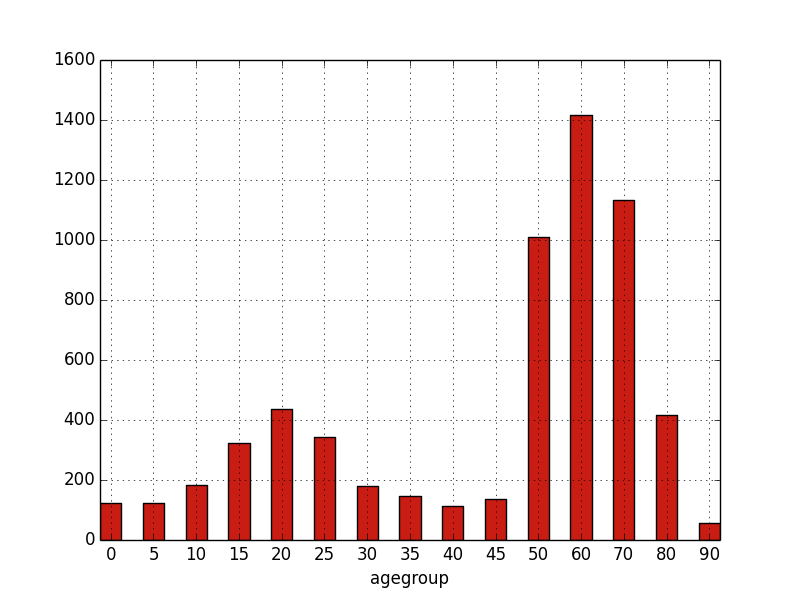
In the first two 1d_expr is (an expression returning) a one-dimensional array (for example an entity field or a groupby expression with only one dimension). For example:
bar(groupby(agegroup))
would produce:
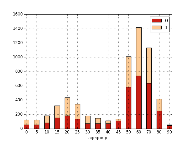
If one passes several arrays/expressions, they will be stacked on each other.
bar(groupby(agegroup, filter=not gender),
    groupby(agegroup, filter=gender))
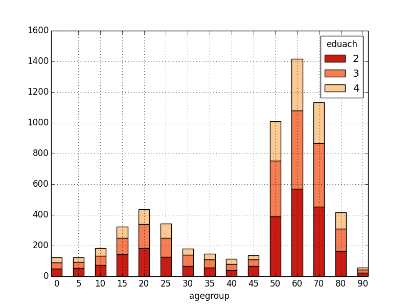
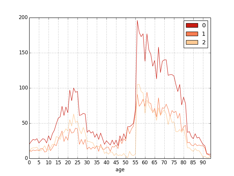
Alternatively, one can pass (an expression returning) a two-dimensional array, in which case, the first dimension will be “stacked”: for each possible value of the first dimension, there will be a bar “part” with a different color.
- bar(groupby(eduach, agegroup))
5.6.6.2. plot
New in version 0.8.
plot can be used to draw (line) plots. It uses matplotlib.pyplot.plot and inherits all of its keyword arguments. There are 4 ways to use it:
plot(1d_expr, ...)
plot(1d_expr1, 1d_expr2, ...)
plot(2d_expr, ...)
plot(1d_expr1, style_str1, 1d_expr2, style_str2, ...)
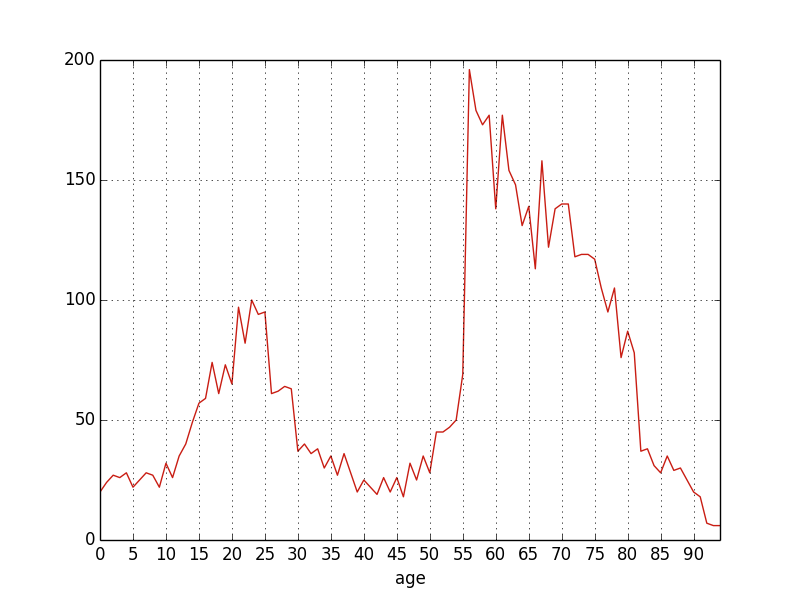
In the first two 1d_expr is (an expression returning) a one-dimensional array (for example an entity field or a groupby expression with only one dimension). For example:
plot(groupby(age))
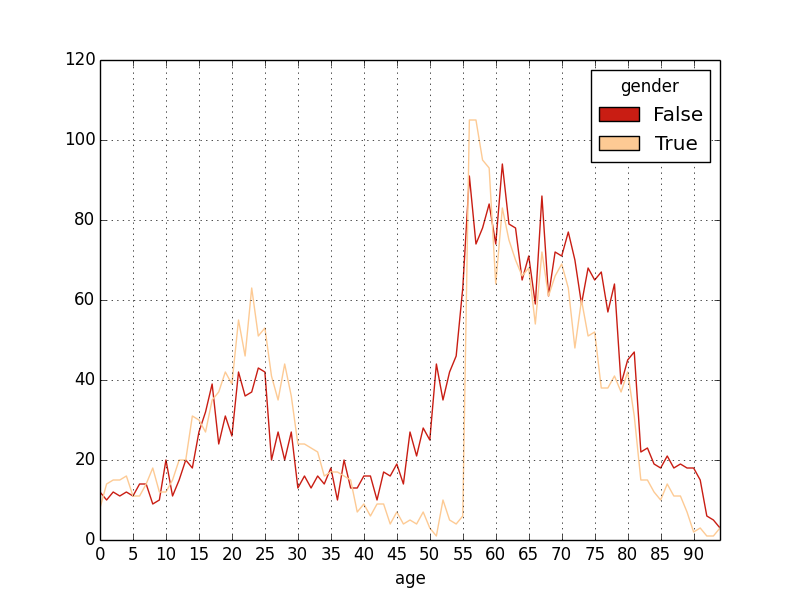
If one passes several expressions, each will be plotted as a different line.
plot(groupby(age),
     groupby(age, filter=not gender),
     groupby(age, filter=gender))
The third option is to pass (an expression returning) a two-dimensional array (plot(2d_expr, ...)) in which case, there will be one line for each possible value of the first dimension and the second dimension will be plotted along the x axis. For example:
plot(groupby(gender, age))
and, using a few of the many possible options to customize the appearance:
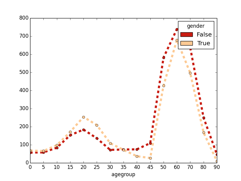
plot(groupby(gender, agegroup),
     grid=False, linestyle='dashed', marker='o', linewidth=5)
And the fourth and last option is to alternate expressions returning one-dimensional arrays with styles strings (plot(1d_expr1, style_str1, 1d_expr2, style_str2, ...)) which allows each line/array to be plotted with a different style. See plot documentation for a description of possible styles strings.
Note
Styles including a color (as explained in the matplotlib documentation – eg ‘bo’) are not supported by our implementation. Colors should rather be set using the colors argument (as explained above and shown in the example below).
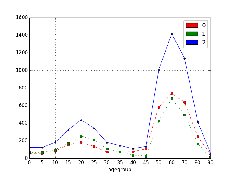
Example:
plot(groupby(agegroup, expr=count(not gender)), 'o--',
     groupby(agegroup, expr=count(gender)), 's-.',
     groupby(agegroup), '*-'
     colors=['r', 'g', 'b'])
5.6.6.3. stackplot
New in version 0.8.
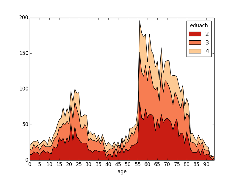
stackplot can be used to draw stacked (line) plots. It uses matplotlib.pyplot.stackplot and inherits all of its keyword arguments. There are two ways to use it:
stackplot(1d_expr1, 1d_expr2, ...)
stackplot(2d_expr, ...)
Example:
stackplot(groupby(eduach, age))
5.6.6.4. pie charts
New in version 0.8.
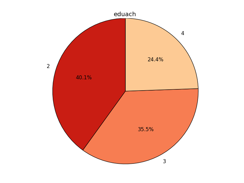
pie can be used to draw pie charts. It uses matplotlib.pyplot.pie and inherits all of its keyword arguments. It should be used like this:
pie(1d_expr1, ...)
Where 1d_expr is (an expression returning) a one-dimensional array (for example an entity field or a groupby expression with only one dimension). Examples:
pie(groupby(eduach))
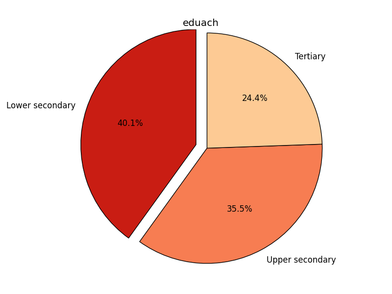
pie(groupby(eduach),
explode=[0.1, 0, 0],
labels=['Lower secondary', 'Upper secondary', 'Tertiary'])
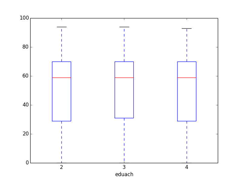
5.6.6.5. boxplot
New in version 0.8.
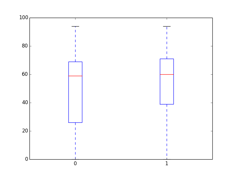
boxplot can be used to draw box plots. It uses matplotlib.pyplot.boxplot and inherits all of its keyword arguments. There are two ways to use it:
boxplot(1d_expr1, 1d_expr2, ...)
boxplot(2d_expr, ...)
Examples:
- boxplot(age[gender], age[not gender])
- boxplot(groupby(eduach, expr=age, filter=eduach != -1))
5.7. Debugging and the interactive console
LIAM 2 features an interactive console which allows you to interactively explore the state of the memory either during or after a simulation completed.
You can reach it in two ways. You can either pass “-i” as the last argument when running the executable, in which case the interactive console will launch after the whole simulation is over. The alternative is to use breakpoints in your simulation to interrupt the simulation at a specific point (see below).
Type “help” in the console for the list of available commands. In addition to those commands, you can type any expression that is allowed in the simulation file and have the result directly. Show is implicit for all operations.
examples
>>> avg(age)
53.7131819615

>>> groupby(trunc(age / 20), gender, expr=count(inwork))

trunc(age / 20) | gender |      |
                |  False | True | total
              0 |     14 |   18 |    32
              1 |    317 |  496 |   813
              2 |    318 |  258 |   576
              3 |     40 |  102 |   142
              4 |      0 |    0 |     0
              5 |      0 |    0 |     0
          total |    689 |  874 |  1563
5.7.1. breakpoint
breakpoint: temporarily stops execution of the simulation and launch the interactive console. There are two additional commands available in the interactive console when you reach it through a breakpoint: “step” to execute (only) the next process and “resume” to resume normal execution.
general format
breakpoint([period])
the “period” argument is optional and if given, will make the breakpoint interrupt the simulation only for that period.
example
marriage:
    - in_couple: MARRIED or COHAB
    - breakpoint(2002)
    - ...
5.7.2. assertions
Assertions can be used to check that your model really produce the results it should produce. The behavior when an assertion fails is determined by the assertions simulation option.
- assertTrue(expr): evaluates the expression and check its result is True.
- assertEqual(expr1, expr2): evaluates both expressions and check their results are equal.
- assertEquiv(expr1, expr2): evaluates both expressions and check their results are equal tolerating a difference in shape (though they must be compatible).
- assertIsClose(expr1, expr2): evaluates both expressions and check their results are almost equal.
![]()
Table Of Contents
- 5. Processes
- 5.1. Assignments
- 5.2. Temporary variables
- 5.3. Actions
- 5.4. Procedures
- 5.5. Expressions
- 5.6. Output
- 5.7. Debugging and the interactive console